1 Introduction

The origin of WebSnapse comes from the Snapse simulator [1] with the following raison d’être: an easy to use and visual simulator for learning about SN P systems. The simulator WebSnapse v1 (that is, version 1) improves on this “reason for being” by allowing users to access the software by using only their web browser, including more animations and features [2]. Unlike Snapse which requires specific installation depending on the device or operating system, WebSnapse is immediately accessible for many devices (including portable ones) and operating systems through their web browsers such as Firefox, Chrome, Safari. Further improvements were introduced in WebSnapse v2 [3], and finally for the present tutorial, the current versions of the simulator available at the WebSnapse page [4]. The interested reader is invited to read the cited works on Snapse and WebSnapse, with links to the simulators, their source codes, etc. at [4].

The present work is organised as follows: we briefly recall the definition of SN P systems (Section 2. In Section 3 we begin the tutorial to the WebSnapse software, focused on its current version. The tutorial involves going through the process of creating an SN P system in detail using WebSnapse. A revised and extended version of the present tutorial is in [5].

2 Preliminaries

A Spiking Neural P (SN P) system from [6] is a tuple \[\Pi = (\{a\}, \sigma _{1}, \sigma _{2}, \dots , \sigma _{n}, syn, in, out),\] where:

• \(\{a\}\) is the alphabet used by the system, and \(a\) is the spike symbol.

• \(\sigma _{i} = (n_{i}, R_{i})\) is the \(i^{th}\) neuron:

  • \(n_{i}\) is the number of spikes contained in the neuron.
  • \(R_{i}\) is the set of rules contained in the neuron. A rule is of the form \[E / a^{c} \rightarrow a^{p}; d,\] where \(E\) is a regular expression over \(\{a\}\), \(c \ge p \ge 0\), \(c \ge 1\), and \(d \ge 0\). A minor modification in the usual way of writing rules in the same (neuron) rule set: we separate rules within the same rule set using vertical bars instead of commas; for instance we write \[\{a \rightarrow a; 1 \mid a \rightarrow \lambda \}\] instead of \[\{a \rightarrow a; 1, a \rightarrow \lambda \}.\]
• \(syn \subseteq \{1, 2, \dots , n\}^{2}\) is the set of synapses, with \((i, i) \notin syn\) for \(1 \le i \le n\).
• \(in\) and \(out\) are the sets of input neurons and output neurons, respectively.

The present tutorial assumes some familiarity of the basics (i.e., syntax, semantics) of SN P systems, such as the chapter dedicated to SN P systems in the handbook in [7], the tutorial in [8], or a recent survey in [9].

3 Tutorial

To demonstrate the simulation of SN P systems, we will create a greater-than-1 positive integer generator \(\Pi _{\ge 2}\), an SN P system that generates the set \(\{k \mid k \in \mathbb {Z}, k \ge 2\}\).

Formally, we have \[\Pi _{\ge 2} = (\{a\}, \sigma _{1}, \sigma _{2}, \sigma _{3}, syn, in, out),\] where:

• \(\sigma _{1} = (2, \{a^{2}/a \rightarrow a; 0 \mid a \rightarrow \lambda \})\)
• \(\sigma _{2} = (1, \{a \rightarrow a; 0 \mid a \rightarrow a; 1\})\)
• \(\sigma _{3} = (3, \{a^{3} \rightarrow a; 0 \mid a \rightarrow a; 1 \mid a^{2} \rightarrow \lambda \})\)
• \(in = \emptyset \)
• \(out = \{\sigma _{3}\}\)

We consider two simulators developed at the Algorithms & Complexity Lab from the University of the Philippines Diliman:

• WebSnapse v3 makes use of code that compiles to WebAssembly in order to efficiently carry out the computations involved when simulating SN P systems [10].
• WebSnapse Reloaded separates the simulator into a client side and a server side, allowing the user to use separate computers to handle the displaying and simulation of SN P systems [11]. In this way WebSnapse Reloaded is also known as WebSnapse CS, for client-server.

For the present tutorial we use WebSnapse Reloaded, as it provides a richer set of features and a more user-friendly interface. The ideas from using WebSnapse Reloaded are transferrable to WebSnapse v3, hence we limit the tutorial to just one simulator. From here onwards we refer to WebSnapse Reloaded as WebSnapse, for brevity.

The reader is recommended to follow the tutorial sections below by accessing the WebSnapse simulator directly using the following link:

Simulation of a system in WebSnapse involves two main steps: (1) creating the system and (2) running the actual simulation of the system.

3.1 Creation

Creating a system can be done in two ways:

1.

Importing or loading an existing JSON file from a previous use of WebSnapse: by simply using the Load button, see Figure 10.

2.

Using the simulator’s user interface to add neurons, rules, and draw synapses between these neurons: we describe these steps in more detail below.

We start by creating \(\Pi _{\ge 2}\) via WebSnapse’s user interface, first adding nodes and then drawing connections between these nodes.

Adding a node involves three steps:

1.

Selecting the Node tool by clicking it or using the keyboard shortcut N (Figure 1)

2.

Clicking anywhere in the canvas to place the node

3.

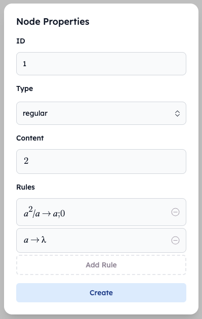
Indicating the node’s properties (ID, Type, Content, and Rules) (Figure  2 and Figure  3):

• ID is a unique identifier for the node, indicated using LaTeX (e.g., n_{1} for \(n_{1}\), env_{out} for \(env_{out}\)). We recommend giving logical or conventional identifiers to nodes for clarity.

• Type is a convention used in WebSnapse: normally a neuron \(\sigma _{i}\) is indicated as an input/output neuron via membership in \(in\)/\(out\), respectively. However, in WebSnapse, \(\sigma _{i}\) is indicated as an input/output neuron via multiple steps:

  • Setting \(\sigma _{i}\)’s type to regular (not input or output)
  • Making a new neuron \(\sigma '_{i}\) and setting its type to input/output
  • Drawing a new synapse \(\sigma '_{i} \rightarrow \sigma _{i}\) (if \(\sigma _{i}\) is an input neuron) or \(\sigma _{i} \rightarrow \sigma '_{i}\) (if \(\sigma _{i}\) is an output neuron)
• The spike count \(n_{i}\) and rule set \(R_{i}\) are indicated just like how the system is defined. Each rule in \(R_{i}\) is typeset using LaTeX, that is, one types or writes on the keyboard \rightarrow or \to for \(\rightarrow \) and \lambda for \(\lambda \), among other conventions.

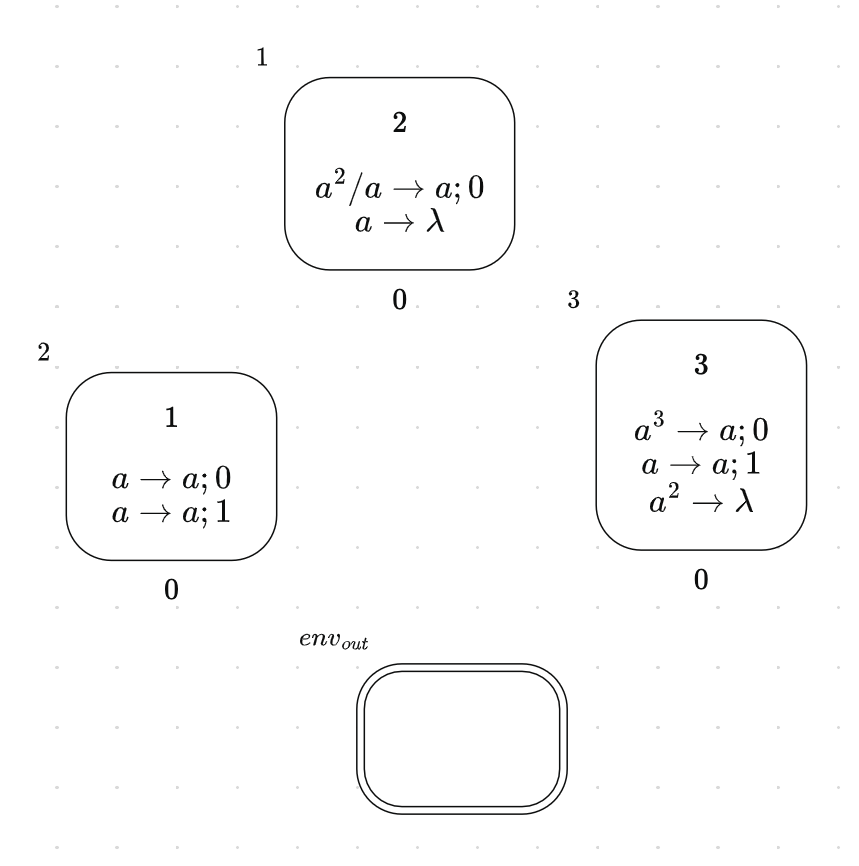
Repeating these steps for each neuron allows us to draw \(\sigma _{1}, \sigma _{2}, \dots , \sigma _{n}\) on the canvas (Figure 4).

Adding a synapse involves three similar steps:

1.

Selecting the Edge tool by clicking it or using a keyboard shortcut: pressing the E key on the keyboard as a shortcut (Figure 5)

2.

Drawing an arc from the synapse’s source node to the synapse’s target node (Figure 6)

3.

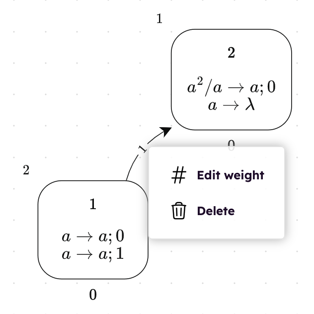
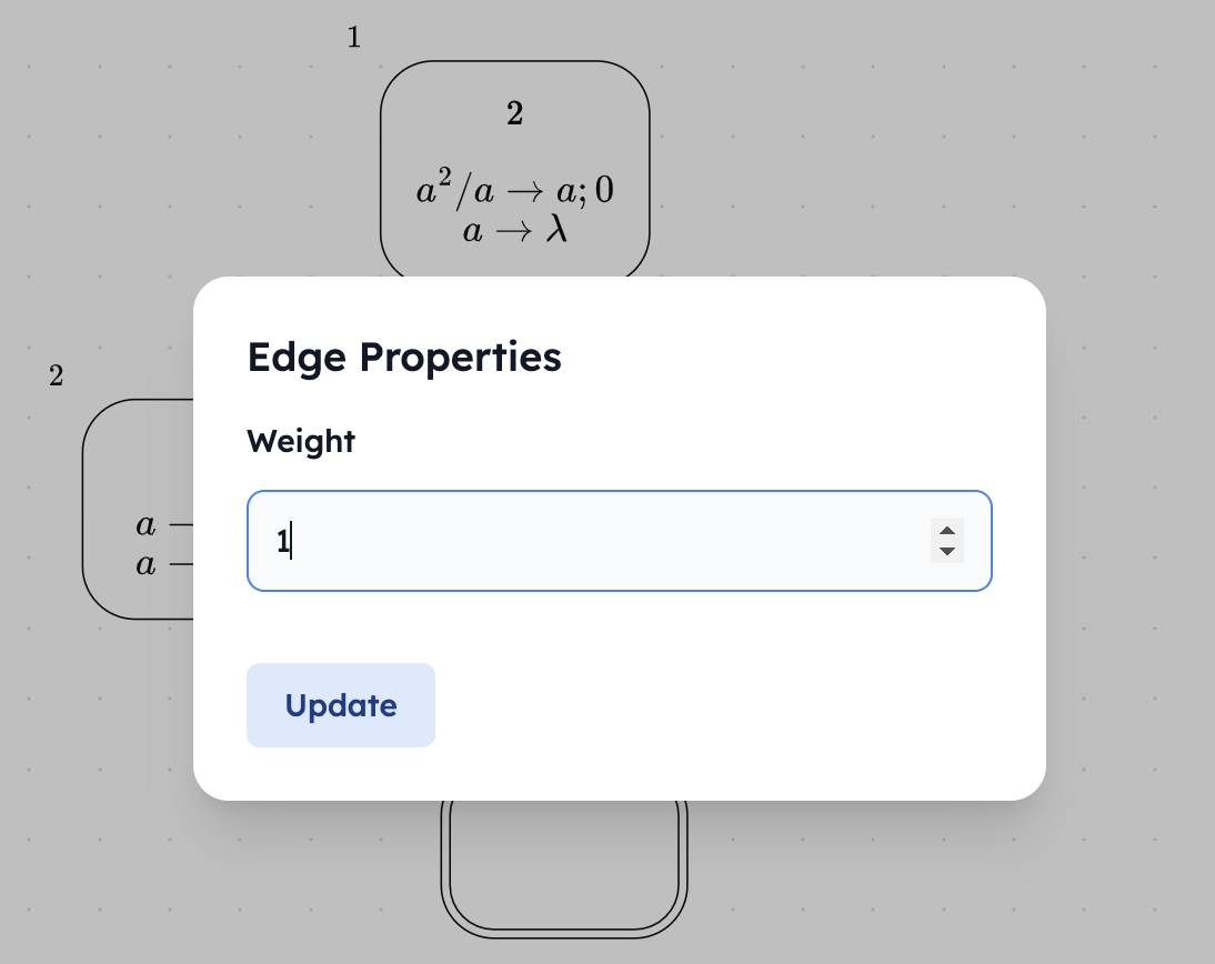
Indicating the synapse’s weight (if necessary; Figure  7 and Figure  8):

• WebSnapse automatically creates a synapse with weight \(1\) after the previous step. To edit the weight, one can right-click on the synapse to make a context window pop up. Clicking Edit weight makes editing the synapse’s weight possible.

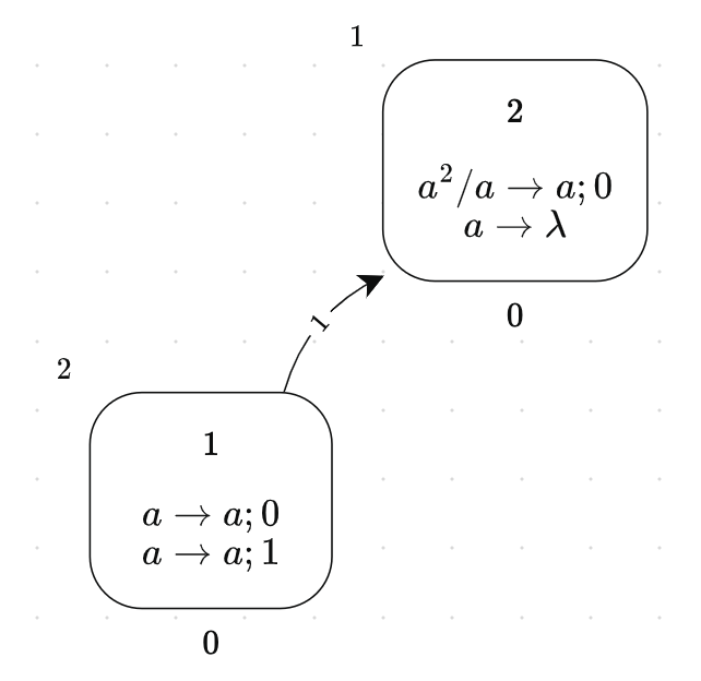
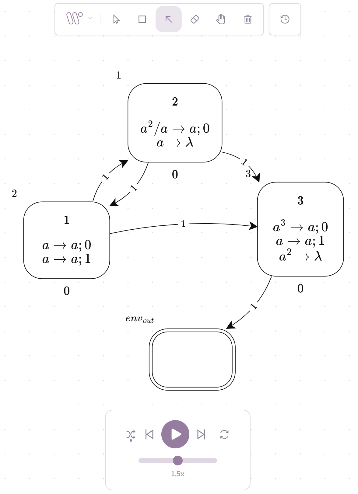
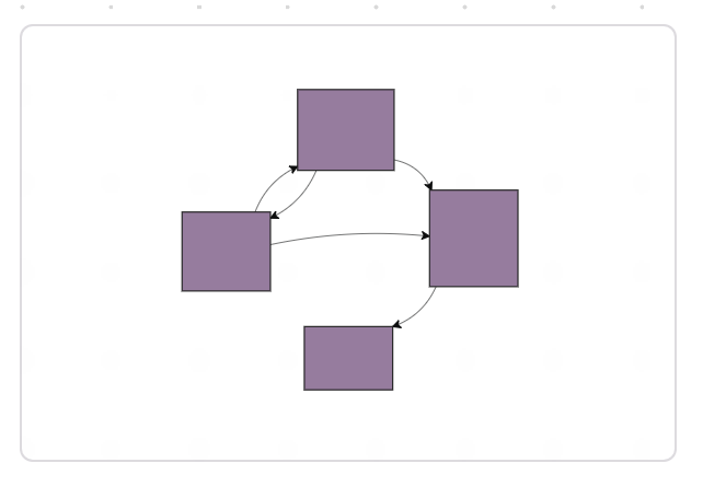
Repeating these steps for each synapse allows us to draw \(syn\), and as a result \( \Pi _{\ge 2} \), on the canvas (Figure 9).

Alternatively, one may create the system by importing a pre-existing JSON file. This is done by clicking on the W-like icon at the top then clicking Load (Figure 10).

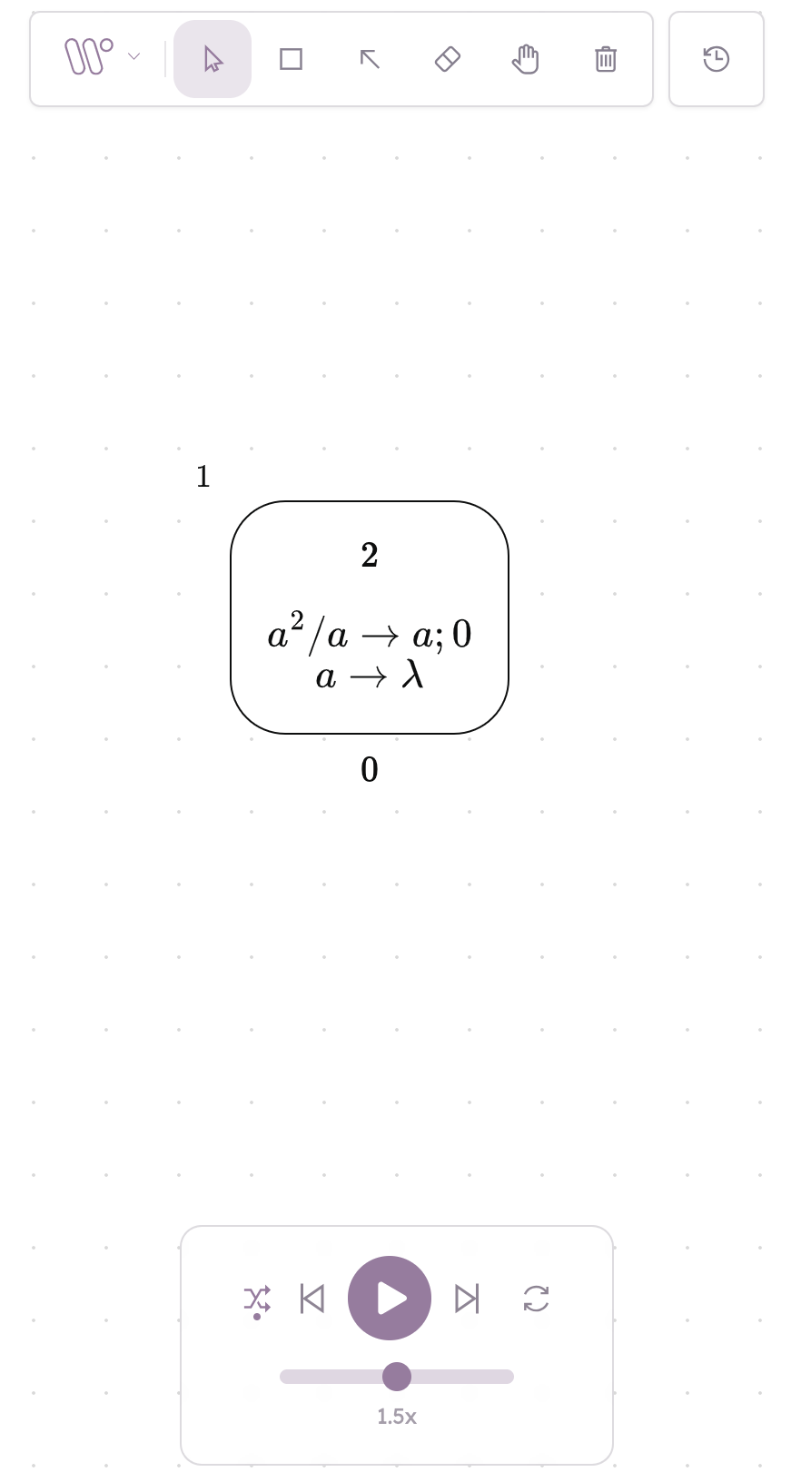
3.2 Simulation

To simulate the system created, we simply click the play button at the bottom of the page. WebSnapse will then simulate each tick of the system, automatically selecting necessary rules and updating spike counts.

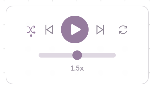
There are several things one may do to control the simulation (Figure 11):

• One may click the icon with crossing arrows (leftmost icon) to toggle between guided and pseudorandom mode. In guided mode, whenever a neuron is capable of activating more than one rule due to nondeterminism, WebSnapse allows the user to decide which rule to activate. On the other hand, in pseudorandom mode, this decision is left to WebSnapse; it will activate one of these rules at pseudorandom.
• One may go one tick forwards or one tick backwards on the global clock of the system by clicking the icons beside the play button. These icons will have no effect if the user has not started the simulation (for the backward button) or if the simulation has finished (for the forward button).
• One may click the icon with arrows in a cycle (rightmost icon) to reset the simulation.

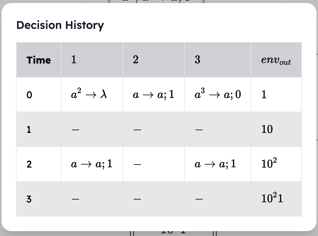
In addition to controlling the simulation and observing how the system behaves, the user may also open the History menu using the rightmost icon on top (Figure 12). This will show the rules selected by standard neurons and the contents of input/output neurons at each time step (Figure 13).

In this way the output of the computation can be taken in two ways: in a “visual” way by checking the contents of the neuron \(env_{out}\) for instance in Figure 9; in a “textual” way by looking at the column for \(env_{out}\) in the decision history (Figure 13. Recall at the start of Section 3 that SN P system \(\Pi _{\geq 2}\) generates, in a nondeterministic way, the number set \(\{ k \mid k \in \mathbb {Z}, k \geq 2 \}\). In the Decision History from Figure 13 we see that at time step (or row) 3, in the column for \(env_{out}\) is the sequence \(10^21\) corresponding to the spike train for the output: the distance or interval between the two “1” symbols is 3, thus the output is \(3 \in \{ k \mid k \in \mathbb {Z}, k \geq 2 \}\).

3.3 Editing

Suppose that instead of \(\Pi _{\ge 2}\), we wanted to create a greater-than-three, multiple-of-three generator \(\Pi _{3k}\), an SN P system that generates the set \(\{3k \mid k \in \mathbb {Z}, k \ge 2\}\). The differences between \(\Pi _{\ge 2}\) and \(\Pi _{3k}\) are subtle; these differences are highlighted in Table 1.

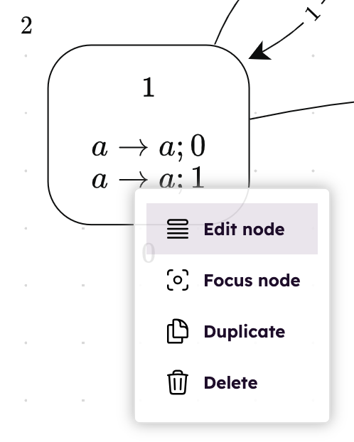
Editing a neuron’s contents is done by right-clicking the neuron to open a context window. Clicking the Edit node option allows one to change a neuron’s spike count and rule set (Figure 14).

In this situation, only the node contents differ between the two systems. In case the synapses also need to be edited, the process is largely the same: one right-clicks the synapse to open a context window, then clicks the Edit weight option to change the synapse’s weight.

3.4 Extras

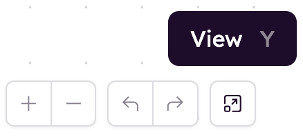
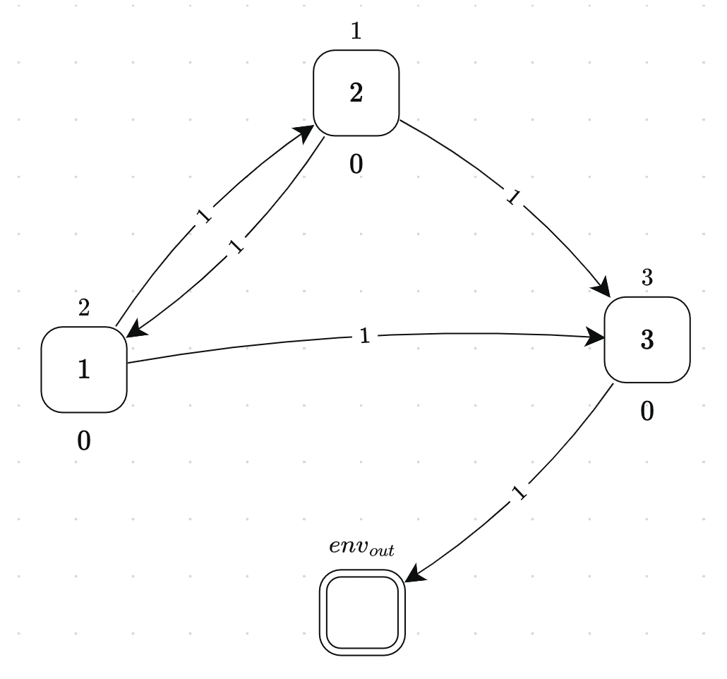
There are several quality-of-life features in WebSnapse that may help the user better understand the system or simulation they are working with. One such feature is the View button on the bottom-left of the screen, which gives the user the option to hide the system’s rules, as shown in Figure 15 and Figure  16.

This is especially helpful when it comes to larger systems with repeated rulesets, for which hiding the rules minimizes the visual clutter on the screen. For instance, the (non)uniform solutions to hard problems in [12] or the homogeneous neurons in [13, 14]. In relation to this, the minimap on the bottom-right of the screen (Figure 17) gives the user a bird’s-eye view of the system, which may help with navigating large systems.

WebSnapse may be extended beyond system creation and simulation. For instance, one may incorporate a routine such as homogenization, as discussed in [13]. An implementation of the homogenisation algorithms in [14] is the following: at least for the WebSnapse v2, work by [15] allows homogenisation using a button click, so that a system \(\Pi \) may be converted to an equivalent homogeneous system \(\Pi '\).

Another possibility for SN P systems is to generate space-filling curves, as discussed in [16] and [17], among others. The robustness of WebSnapse’s codebase makes relevant extensions and features straightforward.

Of course, a simulator is no good if it cannot correctly simulate the systems it is given. In WebSnapse’s development, test cases and scripts were created in order to verify its correctness in both creation and simulation. These test cases found in [4] may also serve as helpful samples for users new to SN P systems or WebSnapse.

4 Final Remarks

This tutorial only scratches the surface of what can be done using both SN P systems and their simulators, but understanding the basic operations and options is fundamental to creating and simulating more complex systems. The user-friendly interface and codebase flexibility of WebSnapse (Reloaded or CS) empower the user to perform these creations and simulations with ease, and to add extensions or new features to the simulator as they see fit. By making good use of simulators such as WebSnapse, researchers are equipped with more guidance and confidence towards exploring the world of SN P systems and P systems in general.

Another way to represent SN P systems and related models is the formal framework from [18, 19] which we hope to support in WebSnapse. Further directions and extensions for WebSnapse, with related theories and tools, are provided in [20] which is a revised and extended version of [21]. Since not only the WebSnapse applications but also their source codes are available in the WebSnapse page in [4], our hope is that more people can use, extend, or improve WebSnapse for their own research. Our group is open to collaborations!

Acknowledgements

Support for F.G.C. Cabarle: the Dean Ruben A. Garcia PCA, and Project No. 222211 ORG from the Office of the Vice Chancellor for Research and Development, both from UP Diliman; the QUAL21 008 USE project (PAIDI 2020 and FEDER 2014-2020 funds). The authors are also thankful to Prof. Gexiang Zhang for suggesting this tutorial, and to the IMCS Bulletin for allowing us to share our work.

References